Self Driving Car

This project is been created without using any libraries.
With this project, we’ll learn about:

• HTML Canvas and how to draw on them.
• How to create a cars and add real world mechanics to it.
• Define roads and its boundaries.
• Create artificial sensors.
• Segment intersection.
• Collision detection and Traffic simulation
• Creating our own Neural Network, Feed Forward Algorithm
• Visualising Neural Networks (or black boxes)
• Optimising our Neural Networks using Parallelisation, Fitness function and Genetic Algorithms (GAs)

1. Canvas and Car mechanics(/physics)

Basic Canvas

• First we create a index.html file and define a <canvas\>. It’s used to draw anything on browser with help of JavaScript
• Linking main.js with the html file.
• myCanvas is the ID for canvas, but as there’s only one canvas, we can use any of them to target the canvas
• Height = window height, and width of 200
• This is a 2d render context (ctx)
• We create a road and a car object

function(animate)
requestAnimationFrame(animate);

This calls the function recursively for like 60 times per second. every time setting height inside this function resets the values of canvas, so no need to ctx.save() or ctx.restore.

Implementation

Car.js

• x and y for coordinates, width and height is self explanatory
  $$Speed, s = \frac{Distance}{Time}$$
  $$Acceleration, a = \frac{\delta v}{\delta t}$$
• Whenever arrow UP key is pressed, we increase the the speed by a factor of acceleration constant and vice versa.
  $$Friction, f = \mu N$$
• If we have any positive speed, we decrease it by a factor of friction, so that a car that has any speed can stop after some time.
• We use angle to translate to the direction of rotation.
• A flip is used so that when car is reversed and rotated, it can use left arrow for left movement and vice versa (making angle negative).

This is a unit circle, We can see when a car is rotated, it should go in the same direction, as its orientation, for that we use

this.x  -=  Math.sin(this.angle)*this.speed;
this.y  -=  Math.cos(this.angle)*this.speed;

So say if a car is at $\alpha = 45\degree$, then x and y increases at same ratio, i.e, $\cos\alpha$ and $\sin\alpha$ increases at same rate, making car go in diagonal $45\degree$. Also multiplying it with speed, for x and y axis in that direction.

Controls.js

This is pretty simple, if a key is pressed, make that direction true, and when lifted, make it false again.

2. Road Defination

Road.js

This is the one which renders the road. It needs x for centering of the elements, and a width. Lane count can be changed as per choice. left and right boundaries
are defined in accordance to x, half of the width to both left and right.

The y-axis is from an arbitrary negative infinity to positive infinity.

Note: Y axis grows/increases downwards

We define borders array, [left, right]. Which takes objects (x, y). Left goes from x at left to y at top, and to x at left and y at bottom.
a. left = 0, top = $-\infty$ to b. left = 0, bottom = $\infty$
c. right = 0, top = $-\infty$ to d. right = 0, bottom = $\infty$

|a		|c
|		|
|		|
|b		|d

getLaneCenter() method gives the centre for any lane index [i=0 -> i=laneCount]

lerp() is a simple method, for linear interpolation, which constructs new data points within the range of a discrete set of known data points. here, we simply passleft,right,t as arguments and depending on value of i, we kinda get a percentage which is usually centred between any lane.

for i=0
LC, lane count = 3
eg. if left = 0, right = 10, $t = \frac{i}{LC}$, then

function  lerp(a, b, t){
return  a  + (b-a) *  t;
}

We can see, $a+(b-a) = b/right$, multiplied by t gives 0 for first time.

for i = 1
t = 3.33, which is at 1/3rd of lane, so we get another data point at $\frac{1}{n^{th}}$ point, here $n = lc$

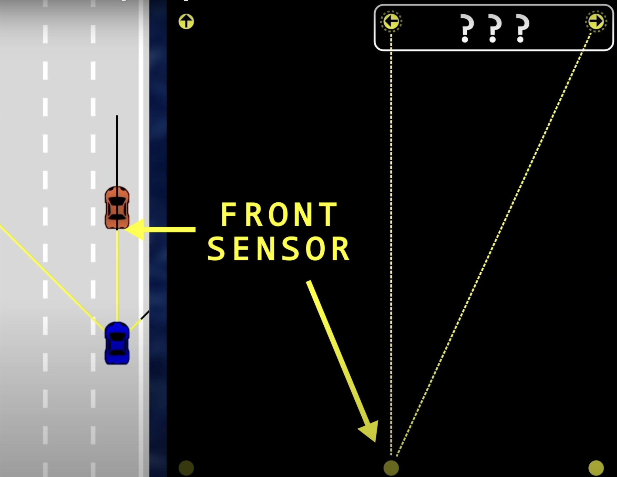
3. Sensors

The constructor for this sensor takes car as an argument. This means it’s car’s sensor. The methods of sensor can be accessed using car.sensor.prototype()

The rayCount specifies no. of rays to be formed, rayLength specifies the length of each ray, raySpread specifies the total angle between the first and last ray,.

rays[] is an array which stores each ray, readings[] is an array that stores the first intersection point for any given ray.

When the car updates to move, we also update the sensors with it.
The update() private method has two things to do, first is to cast rays and second is to get readings from them.

Cast Rays

We again use the utility function lerp() or linear interpolation against each ray.

const  rayAngle  =  lerp(
	this.raySpread/2,
	-this.raySpread/2,
	this.rayCount  ==  1  ?  0.5  :  i/(this.rayCount-1)
)+this.car.angle;

loop i takes values from 0 to rayCount-1 (i.e., excluding rayCount).
For lane, remember, if $lane = 3$, we had 3 lanes, divided into 4 lines, so we took values from 0 to 3, i.e, total 4 values.
But here when we talk about rays, we need only 3 lines (that divides the angle into 2 parts, try to understand, there we referred to the free space, here we talk about borders). Ergo we take values $rayCount - 1$ values.

for rayCount = 3, $t=\frac{i}{(rayCount-1)}$ = $\frac{i}{2}$

This shows we divide the rays into one less no. of parts.

$a+(b-a)*t$

• At $t=0$, ans is $a$, or first ray
• At $t=1$, ans is $a+b-a = b$ or the last ray
• For any intermediate values of t, we get percentage/fractions

We add car’s angle to rotate the sensor with the car.

Note: if rayCount = 1, we can’t divide it into 0 parts, so we pass 50% or 0.5 into lerp function, this will take a value between those two lines exactly at the middle.

Here we have an array, ray. We push into it, start and end points as an array again. x: this.car.x, y: this.car.y basically means the middle point of the car.

const  end  = {
	x: this.car.x  - Math.sin(rayAngle)*this.rayLength,
	y: this.car.y  - Math.cos(rayAngle)*this.rayLength
};

For end points, we basically subtract from coordinates of x and y, the sin and cosines for any angle.
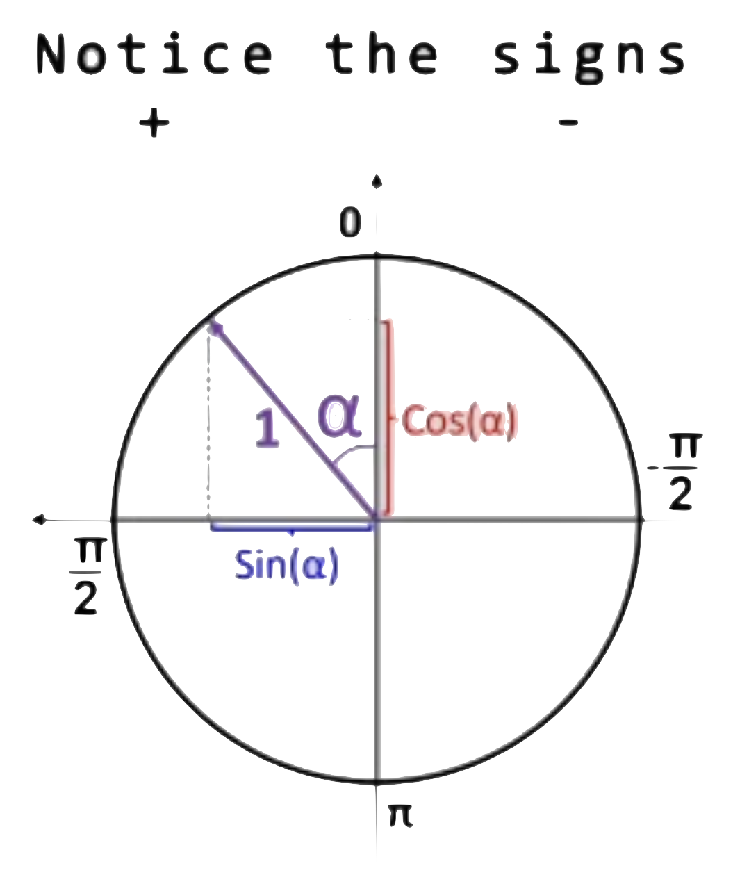
for x, looking at images, angles are positive on left sides, so subtracting from x, we can go left, and if angle becomes negative, the minus sign cancels and makes the x positive.
for y, it same concept, except that y grows positive downwards, so minus sign.
this.rays.push([start, end]); for start, ray[0] and end ray[1].

Get Readings

We pass road borders in following pattern

1. main.js -> car.update(road.borders) (inherits from road.js, borders array)
2. car.js -> upadate(roadBorders), then pass it to this.sensor.update(roadBorders)
3. sensors.js update(roadBorders) passes it to this.#getReading(this.rays[i], roadBorders) which is defined below.

For readings, we need the intersection points, as if where the rays interact with any obstacle, here we take eg of road Borders
For every road border, we pass into getIntersection method, few arguments
it takes, (lineA start, line A end, line B start, line B end)
here our first line, A is our ray, we pass ray[0] to ray[1] which are basically starting and ending points of any ray and start and end of the obstacles, here for $i^{th}$ border.
Then if we have any intersection, we get some values, if not, function returns null. So if it touches any point, we store it in array touches[]
if we have any touch, our Intersection function also returns an offset. So taking advantage of modern js, we use maps to get all the offsets, or distances at which our ray interact, later, we get the minimum offset, because that’s how any real car sensor would work. And then out of all those touches, we return the one with the minimum offset.

Segment Intersection

This is a very important concept to actually calculate the above readings.
If two lines intersect, we need to find the distance of point of intersection from the first line and the second line. Taking advantage of the lerp function, we can assume, that the ratio at which the intersection point divides the first line (say $t$) and second line (say $u$).

Let the ratios be $t$ and $u$.

And the point of intersection be $I$. Let $I_x$ be the x coordinate and $I_y$ be the y coordinate.
Let Line 1 start at $(A_x, A_y)$ and end at $(B_x, B_y)$.
Similarly Line 2 starts at $(C_x, C_y)$ and end at $(D_x,D_y)$
$$I_x = A_x + (B_x-A_x)*t = C_x + (D_x - C_x)*u$$$$I_y = A_y + (B_y-A_y)*t = C_y + (D_x - C_y)*u$$
Taking eq 1
$$A_x + (B_x-A_x)*t = C_x + (D_x - C_x)*u$$$$(A_x - C_x )+ (B_x-A_x)*t = (D_x - C_x)*u$$ let it be eq 3

here $(D_x-C_x)$ can be zero if x = 0, or vertical line.

Taking eq 2

$$A_y + (B_y-A_y)*t = C_y + (D_y - C_y)*u$$$$(A_y - C_y)+ (B_y-A_y)*t =(D_y - C_y)*u$$Multiply the equation with $(D_x - C_x)$ both sides
$$(A_y - C_y)(D_x - C_x)+ (D_x - C_x)(B_x-A_x)*t =u*(D_x - C_x)(D_y - C_y$$
Substituting the value of $(D_x - C_x)*u$ from eq 3, we get
$$(A_y - C_y)(D_x - C_x)+ (D_x - C_x)(B_x-A_x)*t =(D_y - C_y)(A_x - C_x )+ (D_y - C_y)(B_x-A_x)*t$$
Rearranging the terms, (take $t$ terms to one side) and take t as factor, we get.
$$t=\frac{(D_x - C_x)(A_y - C_y) - (D_y - C_y)(A_x - C_x )}{(D_y - C_y)(B_x-A_x) - (D_x - C_x)(B_x-A_x)}$$
We divided it into top (numerator) and bottom (denominator) for better legibility of the code.
We can similarly calculate the value for $u$

$$u=\frac{(C_y - A_y)(B_x - A_x) - (C_x - A_x)(B_y - A_y )}{(D_x - C_x)(B_y-A_y) - (D_y - C_y)(B_x-A_x)}$$Taking minus sign common, we get,
$$u=\frac{(C_y - A_y)(A_x - B_x) - (D_y - C_y)(A_x - C_x )}{(D_y - C_y)(B_x-A_x) - (D_x - C_x)(B_x-A_x)}$$
This way we get same bottom for $u$ and $t$.
The t and u also doubles as offset values, can take any one, let t. They return the distance from origin to point of intersection. As t is again the ratio, we can convert it by taking lerp of (A, B, t) for the exact coordinates.
We also check if $bottom≠0$, and only take values between $0≤t≤1$ and $0≤u≤1$. So we get intersection of line segments (finite) and not line (infinite).

4. Collision Detection

Draw Polygon

Inside car.js, we define a private method, to create a polygon, this polygon really defines the car borders.

#createPolygon(){
const  points  = []
const  rad  =  Math.hypot(this.width, this.height)/2;
const  alpha  =  Math.atan2(this.width, this.height);
points.push({ //top right
x: this.x  -  Math.sin(this.angle  -  alpha)*rad,
y: this.y  -  Math.cos(this.angle  -  alpha)*rad
})

We push an array of points.
First, we define rad or radius of the polygon

We first take the hypotenuse of the polygon
$$rad = \frac{height*width}{2}$$
Then calculate the angle of the corners from the midpoint, say alpha.
$$\alpha = \tan^{-1} (\frac{width}{height})$$

No need to divide by 2, angle remains same subtended to the other corner.

For $x$, we take the $sine$ of the difference of the angles, we know that for top right, angle decreases towards right, so if say the angle is at $0$, we subtract alpha, to move make it negative, to move it right, and right by the angle alpha. Similarly for y, we take $cosine$, of the difference the of the angles, as we know that y increases downwards, so to go up, we subtract alpha.
$$x=\sin(\theta - \alpha)*rad$$$$y=\cos(\theta - \alpha)*rad$$
Multiply by radius ,i.e., hypotenuse, to make the 1px distance to radius px distance.
We adjust the signs accordingly for other coordinates.

Assess Damage

In car.js we define another private method, #assessDamage(roadBorders, traffic) that,
First iterates through every road borders and compares it with every side of the polygon to detect any intersection among both of them.
Similarly it compares with the borders of every side of the polygons for traffic and detects, if it intersects any car in traffic.

We use an utility function for the same, that polysIntersect.
This function takes two polynomials, returns true if they intersect, or touch each other.

const  touch  =  getIntersection(
	poly1[i],
	poly1[(i+1)%poly1.length],
	poly2[j],
	poly2[(j+1)%poly2.length]
)

We use getIntersection method, we go through each side of first polynomial and for every side of second polynomial. Say for a rectangle, i=4, so we go through i=0->1->2->3->0. So we take modulo with the polynomial.length, as there is no 4th index or 5th side, we want to stay inside those values, also, 4%4=0, and a rectangle closes back at first point, so one thing solves 2 problems.

5. Traffic Simulation

We update a lot of things for traffic simulation.

In main.js we create an array for traffic. and generate a new car draw those car in animate() function.
We pass an argument "DUMMY" for traffic cars and "KEYS" for main car. We later go to controls.js and add a switch case to listen for key events for main car only, and that all dummy car always move forward.

We also pass argument for maxSpeed, defaulted at 3, but for dummy cars, we pass 2, so that they move at a slower speed and that our main car can overtake them.

Again in car.js, we don’t draw sensors for cars that are dummy, also while updating sensors, we check that if it’s not a dummy, then only we update sensors that is for the main car.

In main.js when we update traffic cars (basically for drawing, assessing damage and moving them forward), we also don’t pass traffic for damage assess, we pass empty array, so that it doesn’t senses itself and gets damage by itself.

After all of this, we finally modify inside the car.js, the private methods, for sensor and for damage, we pass traffic as arguments, and inside sensors.js , while we update sensors, and get readings, we also pass in traffic for sensors to sense traffic cars as well.

6. Neural Network

We create network.js for this.
Neural Networks are inspired by our brains. Let’s try to break it down.
Neuron are something, that basically holds any number, specifically a no. between 0 and 1. These are all contained in the inputs, outputs, hidden layers. Here we store the offset values for each sensor in first layer, in each neuron respectively. The number/value inside each neurons define its activation. We might call it active when the number is high enough, and deactivated when the number isn’t high enough. That is why we take the $1-offset$ because, less offset, less distance from obstacle is more important.

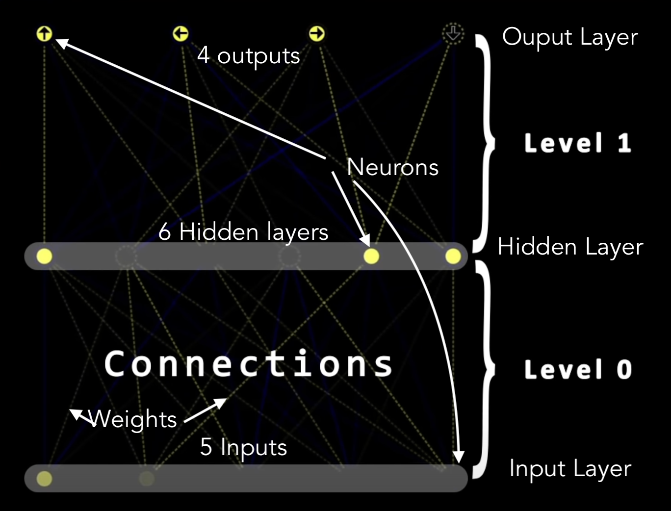
Visualisation of a Neural Network

We have 5 input Neurons one for each ray of the sensor.

Let’s move on to the last layer, it has set of 4 Output Neurons, this specifies each of the forward, reverse, left and right movements, so that car knows, how to move.

We take 1 Hidden Layer with 6 Neurons, and it’s an arbitrary choice.

The way a networks operates, activation in one layer, determines activation in the next layer. And the way how one layer brings the activation in next layer, some group of neurons to generate some outputs, which again acts as inputs for the next layer.

Weights and biases

Here, all 5 of the inputs are connected with all 6 neurons of the hidden layer, so a total of $5*6 = 30$ connections, and each one of those connection have some weights associated with them. Also each output neurons, of every level (not input level) have some biases.

To calculate, let us take all the activation from the previous input neurons and multiply them with the weights of the connection.
Let the activations be $a_1, a_2, a_3, ...a_n$ and the weights be $w_1, w_2, w_3, ... w_n$. And then add all of them, this is called their weighted sum.
$$w_1a_1+ w_2, a_2+w_3a_3+...+w_na_n$$

We have positive as well as negative weights, positive weights influence a output patter to fire, but a negative weight also tells if that particular output does more harm than it helps. Eg, look at below condition, a car should turn, but which way, a negative weight for right turn would easily motivate the car to move left, or else it might hit the border.

We then want this out weighted sum to activate the next neuron, as we know the neurons takes values between 0 and 1, so use some activation functions, such as sigmoid, ReLU, Tanh, Linear, etc to sqeeze the function value to be around this range. Say sigmoid, $\sigma$

$$\sigma(w_1a_1+ w_2, a_2+w_3a_3+...+w_na_n)$$

Then we add the biases (say $b$) to the function, for a neuron to be meaningfully active, say a neuron should only activate if the weighted sum is more than 10, so we add 10 to the function.
That is we want some bias for it to be inactive.
$$\sigma(w_1a_1+ w_2, a_2+w_3a_3+...+w_na_n - b)$$
And that’s just one neuron, all the 5 inputs, connected with all the 6 neurons of hidden layer, $5*6$ weights and next layer, $6*4$ weights, and $6$ biases for first layer, and $4$ biases for second layer. Total of 64 weights and biases.

Machine Learning here really means that finding the right weights and biases.

Simply put,
$$\large a^{(1)} = \sigma(Wa^{(0)} + b)$$

Code

Class Level

This class has some inputs, outputs, weights and their biases. We use a private method #randomize to randomise weights and biases.
These weights and biases in our code are random for now but for a smart brain they’ll have some kind of structure.

Feed Forward Algorithm

This function basically computes for some given inputs, and for that level, the weights of each input and multiply it with the activation of each input, and adds them all, for the weighted sum.
Then it compares if the particular sum is greater than the bias of that neuron, we either make it active or 1 or inactive or 0.
Here we take binary values, but in deep learning networks, these values often have decimal values.

Neural Network Class

It simply creates a new Level according to the Levels passes.
It also has a feed forward method, which calls feed forward method of Level, but also, it makes the current output, as an input for the next level.

We then connect this brain to our car, inside car.js and inside update method we say it to useBrain when car control type is "AI" and set all the outputs to the outputs of the neural network so that it can control our car.

7. Visualising Neural Networks

We create another canvas for this black box, or Neural network, it’s very hard to visualize a neural network with so many dimensions.

Visualizer.js

We define left, top(x, y), width and a height for the canvas. A height for every level as $\frac{total.height}{levels.count}$.
We then use a drawLevel() method to draw our canvas. Here for every inputs and outputs we draw our nodes and connections. We use #getNodeX to get the x coordinates for every neuron space at any level, that again uses our utility function, lerp().

Here we use an interesting thing, that is, Destructuring assignment
const {inputs, outputs, weights, biases} = level, so instead of saying level.inputs or level.baises, we can simply say inputs or biases.

The first for loop draws lines from each input to each output, i.e, the weights. For drawing them, I’ve used an utility function getRGB which takes inputs and gives an RGB value accordingly. For positive activation, we use Yellow (R+G) and for negative values, we use Blue (B).

We used UFT-8 codes for arrow symbols. And set line dashed for drawing the connections.

Animations

networkCtx.lineDashOffset  =  -time/50;
requestAnimationFrame(animate);

This requestAnimationFrame also passes an argument for time, so we use that to animate our line dashes. As the time goes very fast, we divide it by 50, and take negative value of it to make it up, because y increases downwards.

8. Optimising Neural Network

With all of the random neural network, and a single car, we can’t expect some miracle to happen. So we Optimise the code with few methods.

1. Parallelisation

So now we run many different cars, with sensors, and run them all in parallel all at once. Parallel or distributed deep learning can be helpful in reducing the effort taken by high computation. A typical neural network in such intensive computation takes a lot of time to get trained, by parallelisation, we can reduce that time and with our computation power, simulate n number of cars.

We’ll set carCtx.globalAlpha = 0.2; so that all cars remain transparent and set it to 1 for our main car.

Let’s take a look on how do we find our main car, or here we call it the best car.

2. Fitness Function

This is a very important function, it helps us determine what’s the best the best solution is for our car, and actually lets determine the aim for our simulation. It guides our network towards optimal design solution.

bestCar  =  cars.find(
	c  =>  c.y  ==  Math.min(
	...cars.map(c  =>  c.y)
	)
);

Here we define our main objective as to find which car goes the farthest. For that, we first map out from all the given cars, the y axis of all those car, as we know, y decreases upwards, so we take the min of all those car and then use find to actually find which car has that minimum value.

Local Storage for best car.

We create two buttons for save and delete and with that, we can store the best car so that we can resume our progress from there on. We pass it into a JSON format.

But the problem is that, the local storage values are only available to that particular browser, and if you share clone this project, you can’t get the previous results. So we can get that string from console and then store it in a local variable, so that if I share my code with anyone, or run the same project in different browser, I can see my best car with same behaviour across all platforms.

3. Genetic Algorithm (Mutations)

Genetic Algorithms are algorithms that are based on the evolutionary idea of natural selection and genetics. The algorithms follow an iterative pattern that changes with time. It is a type of reinforcement learning where the feedback is necessary without telling the correct path to follow. The feedback can either be positive or negative.

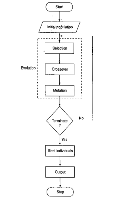
For evolution, we use a method called Mutation. In network.js, we define a method static mutate in Neural Network class, which takes a network and an amount (defaulted at 1 or 100%) as parameters.
We iterate through each level and mutate their weights and biases. Let’s take an example on how we do it for biases.

network.levels.forEach(level  => {
	for(let  i=0; i  <  level.biases.length; i++){
			level.biases[i] =  lerp(
			level.biases[i],
			Math.random() *  2  -  1,
			amount
			)
}

For every level we mutate it’s original biases with help of our utility function lerp() and what we do is take the original value, and set it’s range from a random value of $[-1,1]$ and the amount is value of mutation. The less it is (closer to 0) the less our bias deflect from original, the more it is (closer to 1) the more randomised our biases get, i.e., equal to that random value.

We do the same for weights as well

So what really happens is consider we have our best car which crosses some obstacle but isn’t able to cross certain obstacle. So say the car is almost crossing that obstacle but misses it by an inch. What we do is set a very low value for our Mutation, say 0.1. This will help randomise our remaining cars to shift a little bit here and there so that we can finally go through that obstacle.

But now consider a situation, where the car is very far away from crossing that obstacle, so we set an higher value for our mutation, so that cars get more randomisation and crosses the obstacle somehow.

Ergo, a lesser value for mutation will result in more cars be like our original car, and more value of mutation will lead to less cars follow footsteps of our original car.

From this we select ( or save ) the best car and after successful results, we can finally stop parallelisation and mutations and can get one single car that can do it all.

---

Guided by Dr. Radu Mariescu-Istodor, Lecturer in Computer Science at Karelia University of Applied Sciences.
Course Details
Website

The End